Methods of Calculation.

The Model.

In this program, the Lennard-Jones (6-12) potential is used to model the interaction between molecules. It was tested on various diatomic molecules and proved to be quite accurate.

The Method.

The equation for calculating the second virial coefficient for a diatomic Lennard-Jones molecule could be found in [3] page 144 which is:

where V is the volume and omega is the normalizing factor which depends on the number of angular variables need to specify the orientation of the molecule (Galassi et. al. ). In this method, the variable omega² is equal to the number of rotations performed at a given distance.

Instead of numerically integrating the expression for the second virial coefficient given above, the integral is evaluated as follows:
The inner integral which involves the orientation of the two molecules is calculated by randomly rotating the two molecules around their center of mass. For a given rotation the potential energy between the two molecules and the value

f(r) = [ exp(-U(r)/kT)-1 ]
is calculated. After a large number of rotations, the average value of f(r) is a value for the inner integral. After obtaining the values f(r)*r*r versus separation distance (r), the outer integral could be performed numerically to give a value (call it "I") and by using

B(T) = -2*Pi*N_A*I
where N_A = Avogrado's number
gives, after the appropriate unit conversions, the value for the second virial coefficient.

The Program.

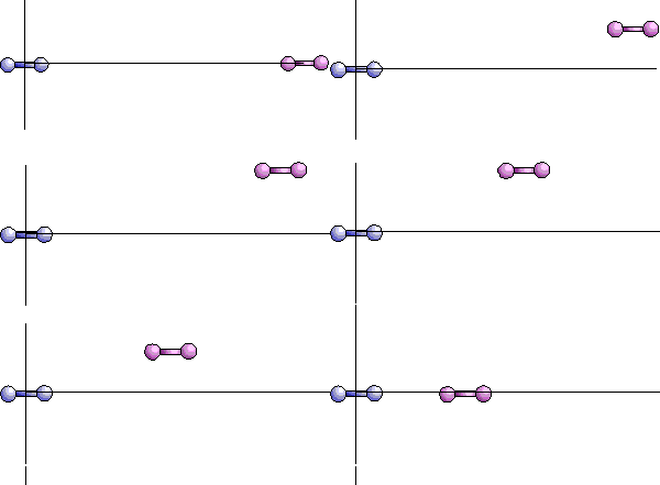
The program contains one input file, one executable file, and generates two output files. The executable file first reads in data from the data file called "b2data.dat" . Then it positions the two groups according to the starting coordinate. Next, the program calculates the coordinates of the two molecule's center of mass. The program then moves the first molecule and positions its center of mass at the orgin. The second molecule is also moved and placed at the same separation distance and orientation.

Once the two molecules are positioned relative to the origin, the second molecule is moved in and place at a distance read in the input file.

Click to move molecule 2

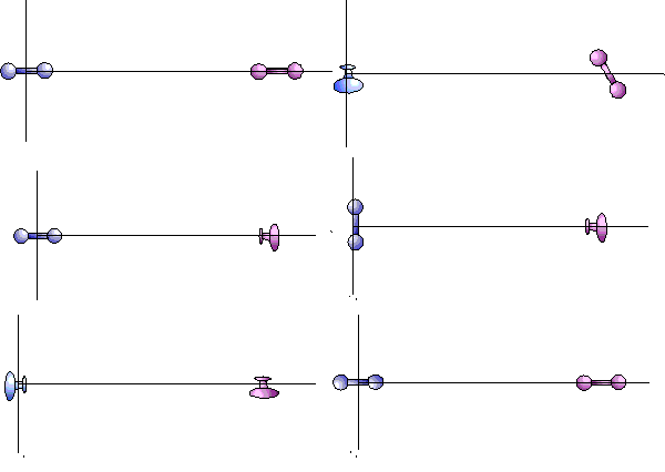
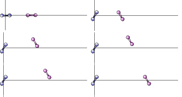
Each molecule then randomly chooses an axis (x,y, or z) to rotate about by a random amount theta. After each molecule has rotated, the potential energy between the two configurations is calculated using the Lennard-Jones 6-12 potential. Also, the quantitiy
f(r) = [ e^-U/k_BT- 1 ] is recorded.
Click to rotate the two molecules.

The rotation and energy calculation is repeated for a desired amount depending on the separation distance and interactions. The input file allows us to set four different amounts of rotation trials according to the separation distance. After completing the task, it then calculates the average of f(r), and the value of r and f(r)*r² are stored in the file "rvsf.dat".
Click to move molecule 2 outward.

Once all of the above has been done, molecule 2 is then moved outward at an increment indicated in the input file. Then, the whole process of rotation and energy calculation is repeated until the maximum separation distance is achieved.

When the maximum distance is reached, the program opens the file "rvsf.dat" and uses Simpson's rule to integrate the data points. Click here to see a typical plot of the file "rvsf.dat". Another purpose for plotting out the file is that it shows where rapid changes occur. At greater distances, the curve falls off quite rapidly and then levels out. From there, we can indicated where small increments are not necessary and so larger distance increments can be used without causing substantial errors when integrating. The value of the integral has units of (A³/mol) so it must be converted to the more accepted (cm³/mol).
Top of Page

Input file A typical input file looks like this, with the bold characters representing input values. :

Data for second virial coefficient calculation
[1] Enter type of molecules being calculated
	'pure fluorine'
[2] Temperature (K):
143.15  
[3] Number of group 1 beads.
2  
[4] Number of group 2 beads.
2  
[5] Coordinates and mass of the group1 beads:
TYPE      mass          x	 y	z
1          14          0.0      0.0    0.0      
1          14          1.089      0.0    0.0    
Coordinates and mass of the group2 beads:
TYPE      mass           x	y	z
1 	   14           9.0     0.0     0.0     
1     	  14          10.089    0.0     0.0    
[6] Number of rotation trials for first to forth interval. 
Starting distance (A)		Number of rotations.
	0			1000
	2			1000
	6			1000
	15			1000
[7] Number of Hamiltonians.
1
[8] Number of LJ groups.
1
[9] Rank 3 array of sigma's(Angstrom) and epsilon/k's(K)
for each hamiltonian. Start new line for new hamiltonian.
	      sigma 11, 22, ...		            
		  3.298  	
	      Epsilon 11, 22, ...
	         36.2	
[10] kappa_ij (Correction to Berthelot rule): eps_ij=sqrt(eps_1*eps_j)*(1-kappa_ij)
Enter in order (1,2) (1,3) (1,4) (2,3) (2,4) etc. Start new line for new Ham.
 0
[11] lambda_ij (correction to Lorentz rule) : Sig_ij=0.5*(sig_i+sig_j)*(1-lamda_ij)
Enter in order (1,2) (1,3) (1,4) (2,3) (2,4) etc. Start new line for new Ham.
 0
[12] Maximum distance between the two groups (Angstrom).
60
[13] Length of normal increments.
0.2
[14] Value of small increments during rapid changes.
0.05
[15] Maximun distance before ending small increments (Angstrom).
15

Details of the Input file.

[1] Type of simulation (can hold up to 20 characters).
[2] Temperature of interest in Kelvins.
[3] Number of atoms in molecule 1.
[4] Number of atoms in molecule 2.
[5] Starting coordinates of molecules 1 and 2. The two could be place anywhere in 3D space with any separation distance. Setting them on the x-axis is purely for covenience.
[6] Adjust the number of rotations for a given distance. The purpose of this is that we can increase the number of rotaion where the interactions are significant and decrease them where changes are not so rapid (such as when the molecules are far from each other). This greatly reduces the computational time.
[7] Number of Hamiltonians. However, this option is not yet functional. Hamiltonian equals 1 is used.
[8] Number of Lennard-Jones Groups.
[9] Arrays of epsilon/k_b and sigma. Only need values for pure components. The values for mixtures are later calculated.
[10] Correction to Berthelot rule.
[11] Correction to Lorentz rule.
[12] Maximun separation distance between the two groups (Angstrom).
[13] Longer increments which are used where changes are not so aprupt.
[14] Smaller increments used where changes in the function are rapid.
[15] Distance where transition from small to large increments occur.

Top of Page.

Results File.

A typical output (results) file looks like this:

Results file for second virial coefficient calculation
 
 Calculation for molecule type : pure fluorine       
 
 Temperature =  143.1499939 K
 
 Epsilon/k (K) =  36.20000076
 
 Sigma (Angstrom) =  3.298000097
 
 Maximum distance evaluated is at r =  59.85020447  Angstrom 
 
 Number of rotations from  0.0000000000E+00 to 2.000000000  =  1000
 
 Number of rotations from  2.000000000 to 6.000000000  =  1000
 
 Number of rotations from  6.000000000 to 15.00000000  =  1000
 
 Number of rotations from  15.00000000 to 59.85020447  =  1000
 
 Number of data points integrated:  525
 
 Small increment =  0.5000000075E-01  Angstrom starts at 0 and changes
 to increment =  0.2000000030 at r =  15.05003929  Angstrom
 
 The value of the integral is  19.47787666
 
 The reduced value (B*) of the second virial coefficient is  -1.628961682
 
 The value of the second virial coefficient is  -73.69910431  cm^3/mol

The reduced value (B*) is defined as :
B^* = B(T)/(2/3*pi*sigma³)
Top of page.