Gibbs Project

CO₂-H₂O

Contents

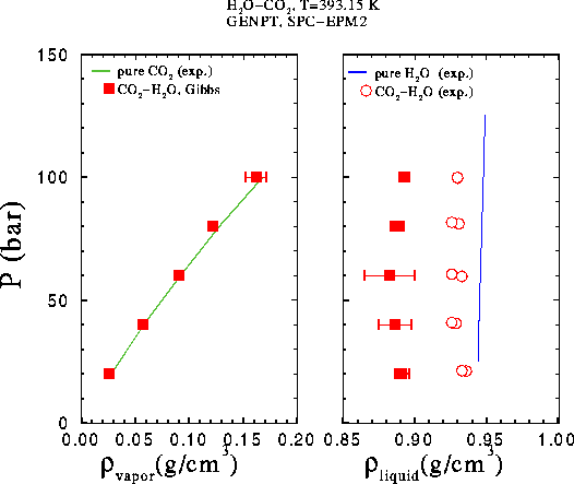
Comparison of simulation data with experimental results. The EPM2 model was used^* for carbon dioxide (see also results for CO₂), water was modeled using the SPC model (see also results for H₂O).

• Phase envelope at low temperatures and moderate pressures
• T = 348.15 K, p = 25 bar - 300 bar
• T = 373.15 K, p = 25 bar - 300 bar
• T = 393.15 K, p = 20 bar - 100 bar
• Short summary
• Phase envelope at high temperature and high pressures
• T = 523.15 K, p = 200 bar - 2000 bar

Several points on the phase envelope were calculated using Gibbs1.11 (Theodorou and Suter method for the LJ interactions). Experimental data for the composition of the liquid phase at this temperature were calculated from Wiebe and Gaddy, J. Am. Chem. Soc., 61, 315 (1939), an estimation for the composition of the vapor phase was made using data from Wiebe, Chem. Rev., 29, 475 (1941). Experimental data vor the densities were not available. The system size was N = 250, the runs took from 3 to 4.5 million configurations.

• p(rho)
  Graph / Numbers
  Since the concentration of water in the gas phase is relatively small the density of the gas phase is approximately the same as the vapor density of pure carbon dioxide. The same is valid in the liquid phase which consists mainly of water. Therefore the liquid density of the binary is underestimated because the SPC model underestimates the liquid density of pure water.
• p(x_CO2, y_CO2)
  Graph / Numbers
  The simulation results agree with the experimental data for the solubility of CO₂ in H₂O within the statistical uncertainties with the exception of the point at 75 bar. The minimum of the solubility of H₂O in CO₂ between 100 and 150 bar is not found in the simulation but the concentration of the gas phase below 100 bar is probably evaluated correctly within the statistical uncertainties.
  Note: Especially for the compositions of the vapor phase there are small differences between the data calculated from Wiebe, Chem. Rev., 29, 475 (1941) and the experimental data of Zawisza and Boguslawa, J. Chem. Eng. Data, 26, 388 (1981) (liquid), Sako et al., J. Chem. Eng. Jpn., 24, 449 (1991) (liquid/vapor), and Coan and King, J. Am. Chem. Soc., 93, 1857 (1971) (vapor). Click here to see a "summarized" graph.

T = 373.15 K, p = 25 bar - 300 bar

Several points on the phase envelope were calculated (Gibbs1.11). Experimental data for the composition of the liquid phase were calculated from values by Wiebe and Gaddy, J. Am. Chem. Soc., 61, 315 (1939) resp. taken from Zawisza and Boguslawa, J. Chem. Eng. Data, 26, 388 (1981), data for the composition of the vapor phase were taken from Coan and King, J. Am. Soc. 93, 1857 (1971) and Tödheide and Franck, Z. Phys. Chem. Neue Folge, 37, 387 (1963). No experimental data for the densities were available.

• p(rho)
  Graph / Numbers
  As one would expect, the situation is the same again, the vapor densities agree essentially with the density of pure CO2, the liquid density is underestimated.
• p(x_CO2, y_CO2)
  Graph / Numbers
  The simulation results agree with the experimental data for the solubility of CO₂ in H₂O within the statistical uncertainties with the exception of the point at 300 bar. It is likely that also this isotherm goes through a solubility minimum but due to the lack of experimental data between 100 bar and 150 bar it is not quite clear where this takes place. Again, the solubility of H₂O in CO₂ up to 100 bar would probably agree with experimental data within the statistical uncertainties.

GEMC-NPT runs with N = 350 particles were carried out and the results compared with data by Nighswander et al., J. Chem. Eng. Data, 34, 355 (1989). The length of the runs was 4 million configurations, all results except the point at 20 bar were obtained using Gibbs0.9 (constant cutoff radius for the LJ interactions), the point at 20 bar was calculated using Gibbs1.11.

• p(rho)
  Graph / Numbers
  Again, the density of the gas phase is again approximately the same as the vapor density of pure carbon dioxide. The experimental data show that the density of the liquid phase of the binary is only slightly smaller than the density of pure water. Since the SPC model underestimates the liquid density of pure water it underestimates the liquid density of the binary, too.
• p(x_CO2, y_CO2)
  Graph / Numbers
  Very good agreement with experiment for the solubility of carbon dioxide in water is found, the concentration of carbon dioxide in the vapor phase is slightly underestimated.

CO₂-H₂O at low temperatures and moderate pressures

The simulation results for the solubility of carbon dioxide in water agree with most of the experimental points for the liquid phase within the statistical uncertainties. Since the influence of the temperature on the gas solubility in water is very small these deviations could not be described by the simulations because the statistical uncertainities cover the whole range of the differences. In the vapor phase the agreement of simulation and experiment in the pressure range up to 100 bar is quite good, the minima of the solubility of water in carbon dioxide between 100 bar and 150 bar could not be seen , though. The trend that with increasing temperature the amount of water in the vapor phase increases is also found in the simulations.

T = 523.15 K, p = 200 bar - 2000 bar

In order to get an idea of the rho(p)-behaviour of the pure (model-)components CO₂ and H₂O at high pressures constant NPT simulations were carried out at T = 523 K. As one would expect the density of pure water is underestimated (approx. 13% at lower pressures, around 6% at higher pressures) by the SPC model. Although the SPCE model shows better agreement with the liquid densities the SPC model was chosen for representing water since it gives the better vapor pressures (see also results for H₂O). Again, the EPM2 model gives good agreement with the experimental densities.
In the system CO₂-H₂O at some pressure the vapor phase becomes more dense than the liquid phase. (The number density of the vapor phase is still lower than the number density of the liquid phase, the vapor (rich in CO₂) reaches the higher density just because of the higher molecular weight of CO₂). In the simulation the density inversion for the pure components takes place at a pressure around 1450 bar while from experimental data one would expect this to happen at a pressure around 1600 bar.
Although the results for the pure components are promising the investigation of their binary at high pressures and temperature turned out to be much more difficult than expected. GEMC-NPT runs were carried out and the results compared with the experimental data by Tödheide and Franck, Z. Phys. Chem. Neue Folge, 37, 387 (1963) resp. Takenouchi and Kennedy, Am. J. Sc., 262, 1055 (1964).
The results of the different authors are in quite good agreement only for the solubility of CO₂ in H₂O but differ up to 12 mole % for the concentrations of H₂O in the vapor phase.
First, several points on the phase envelope were evaluated using Gibbs0.9. Relatively big system sizes (N = 400 - 600) were used to run under those conditions to avoid program stops due to the fact that the length of one of the simulation cells becomes smaller than the cutoff (because of the high densities of the phases). The runs took up to 7 million steps.

• p(rho): Regarding the trend of the densities the liquid densities at the pressures 400 bar and 900 bar are probably off. The vapor density of the mixture follows essentially the curve of the vapor density of pure fluid since (again) the vapor phase contains mainly CO₂. Several attempts were necessary to get the point at 900 bar because the simulation was carried out of the two phase region. A run at a pressure of 600 bar was still not equilibrated after 5 million configurations. The inversion of density takes place at 1500 bar, experimentally this is expected at a pressure of approx. 2000 bar (Tödheide and Franck). Numbers
• p(x_CO2, y_CO2): The concentrations show strong scattering, especially the point at 900 bar seems to be off. The densities at 1200 bar were still not equilibrated after 5 million configurations. In general the concentrations seem to follow rather the experimental curve by Tödheide and Franck than the results from Takenouchi and Kennedy. Numbers

One reason for the scattering of the above mentioned results might be that runs under these conditions need a very long equilibration period, especially when the number densities of the two simulation cells become very similar. Therefore a second attempt to calculate the phase envelope of CO₂-H₂O was made by running Gibbs1.11 with a smaller system size of N = 250. The runs took between 4 and 5.5 million steps.

• p(rho): The density inversion of the binary takes place at approx. 1750 bar. Numbers
• p(x_CO2, y_CO2): (Runs are continued at the moment). Numbers

Note: According to the potential parameters reported in Harris and Yung, J. Phys. Chem., 99, (1995) the cross parameters sigma_C-O were calculated using the Berthelot combining rule sigma_C-O=sqrt(sigma_C*sigma_O)*(1-k_ij) instead of using the usual Lorentz rule sigma_C-O=1/2*(sigma_C+sigma_O)*(1-l_ij) which lead to a slight correction of the Lorentz rule (l_ij=0.001036). This correction was removed in the meantime since its influence lies within the statistical uncertainties.

Last modified by Johannes, August 21st 1996
Page created by Johannes, August 1st 1996